Project Lead: Sean Kearney
Project Type: Dissertation, PhD Soil Science (Faculty of Land and Food Systems)
Supervisors: Dr. Sean Smukler, Dr. Kai Chan, Dr. Nicholas Coops
Project Partners: The United States Agency for International Development (USAID); The Earth Institute at Columbia University, NY; The International Center for Tropical Agriculture (CIAT); Programa Salvadoreño de Investigación Sobre Desarrollo y Medio Ambiente (PRISMA)
Background and Rationale
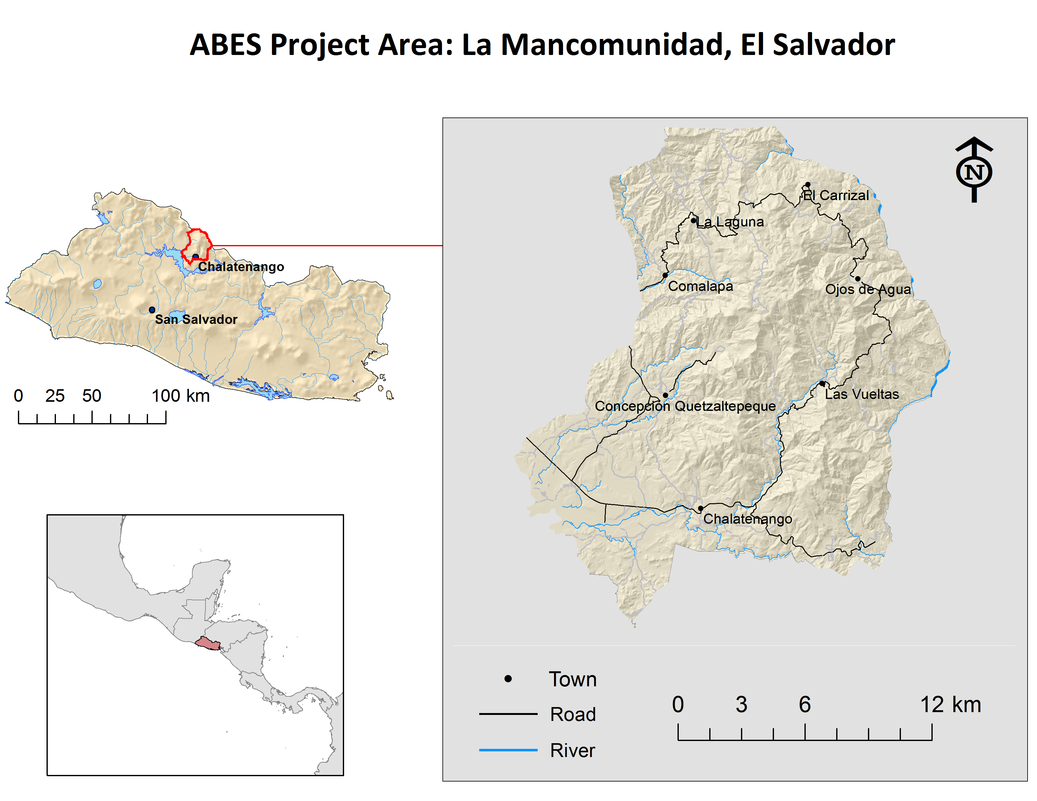
Map showing the entire ABES project area, encompassing La Mancomunidad de la Montañona
Sean’s PhD research is part of the USAID-funded project Agroforestry for Biodiversity and Ecosystem Services (ABES). A collaboration between the Earth Institute, CIAT and PRISMA, the project is investigating the adaptation of a slash and mulch agroforestry system (SMAS) to El Salvador. The SMAS was originally developed in Honduras (known as the Quesengual slash and mulch agroforestry system) in the early 1990‟s and with the participation of farmers, Food and Agriculture Organization (FAO) and other institutions, has been adopted by over 10,000 farmers covering at least 10,000 ha in Honduras, Guatemala, Nicaragua and Mexico. The purpose of this project is to assess the potential for slash and mulch agroforestry systems to increase farm productivity, profitability, and capacity to adapt to climate change and impact landscape biodiversity and other ecosystem services through a combination of on-farm field studies, landscape inventories and remote sensing analysis in a mountain agricultural region in north-central El Salvador. More information on the ABES project can be found at:www.abesproject.org.
Interest in quantifying ecosystem services in developing countries is growing in the face of an increasingly volatile climate and the emergence of opportunities to compensate smallholder farmers for sustaining ecosystem services. Yet monitoring ecosystem services in heterogeneous landscapes remains a challenge. Within the ABES project, I am carrying out research efforts to integrate comprehensive field sampling and high-resolution satellite imagery to quantify a variety of ecosystem services, including soil fertility, carbon storage in both soils and woody biomass, biodiversity and erosion mitigation. With the objective of improving landscape-scale modeling, a multi-scale research approach is underway with data collection at the plot, farm and watershed scales. I am seeking to improve on methods to balance efficiency and accuracy and integrating the use of Fourier-transformed mid-infrared spectroscopy for soil analysis, allometric equations for biomass estimation and erosion pins for monitoring soil loss. Geospatial modeling will be used to develop high resolution land use/cover maps, contiguous digital soil and carbon maps and identify hotspots of biodiversity and degradation. At the nexus of emerging technologies in soil science, land change science and geo-spatial modeling, this research seeks to provide results critical to decision-making for a variety of stakeholders, while furthering our understanding of ecosystem service dynamics in smallholder landscapes.
Objective
To further develop methods to accurately and efficiently monitor ecosystem services at the landscape scale in heterogenous smallholder landscapes.
Research Questions
The goal of this research project is to evaluate ecosystem service indicators related to carbon storage and soil quality. Existing and potential carbon stocks in aboveground woody biomass and soils will be mapped and modeled to better understand the landscape and identify the potential for climate change mitigation. Soil fertility for agricultural production will be assessed with a focus on identifying soil management zones. Finally, the impact of widespread adoption of a “slash and mulch” agroforestry system on these ecosystem services will be investigated. While my exact research questions are still in development, the following are examples of the types of questions I plan to explore:
Related to carbon stocks:
- What is the existing amount of carbon stored in the soil and woody biomass of forests and various managed land uses (e.g. agroforests, live fences, wooded pastures)?
- What are the tradeoffs in costs and uncertainty associated with methods used to map carbon stocks at the landscape scale? Specific methods to be evaluated include the use of LiDAR, very high resolution satellite imagery (e.g. QuickBird), and medium-resolution imagery (e.g. RapidEye, Landsat).
- What is the potential for increasing carbon stocks at both the farm and landscape scale through land management?
Related to soil quality:
- Can soil properties be mapped at the landscape scale with sufficient accuracy to support land management decisions?
- If so, can useful soil management zones be identified to provide recommendations to maximize productivity while minimizing environmental degradation?
Related to slash and mulch agroforestry systems:
- What is the impact of slash and mulch agroforestry on carbon stocks and soil quality at the farm scale?
- What would be the potential impact at the landscape scale under various adoption scenarios?
- Is there a significant climate change mitigation potential with the adoption of this system? If so, is it feasible to promote this system through carbon financing?
- Are there priority areas within the landscape where slash and mulch agroforestry or other land management strategies should/could be promoted?
Methods
The first step in this research project was to carry out a baseline landscape assessment (BLA) to collect field data relevant to quantifying various ecosystem services. Fieldwork for the BLA is complete and data analysis is currently underway and nearly finished. Below is a general overview of the methods employed to collect data in the field for the BLA. More information on the methods used for data analysis and other aspects of this research project will be included in the near future.
Sampling for a baseline landscape assessment (BLA) was carried out from November 8 to December 19, 2012. A total of 144 plots where sampled within a 100 km2 area in northern El Salvador. The project area encompasses La Mancomunidad de La Montañona, located about 2 hours north of San Salvador near the city of Chaletenango and centered around the town of Las Vueltas.
Sampling was carried out using a methodology adapted from the Land Degradation Surveillance Framework (LDSF) developed by the Africa Soil Information Service (AfSIS) to provide a standardized and low-cost methodology for soil and land use monitoring and digital soil mapping around the world (Vågen et al. 2010). The LDSF uses a hierarchical sampling protocol that distributes sampling sites across a landscape in clusters to maximize spatial coverage while minimizing field sampling costs. This enables soil and vegetation sampling across challenging landscapes. The hierarchical design results in a total survey area of 100 km2. Within the survey area, 16 clusters were established, each with a coverage of 1 km2. Each of the 16 clusters is then comprised of up to 10 plots with an area of 0.1 ha (or 0.001 km2) within which subplots of 0.01 ha were established for select data collection.

Clustered sampling within the 100-square km BLA project area
The figure below shows the layout of each of the plots sampled within the BLA. Each plot has a radius of 17.84 m (1000 m2). Within each plot are four subplots that are used to collect soil samples and herbaceous and shrubby vegetation data. All general plot data is taken from the center point (1) including landform, slope, topographic position, land designation, etc (described in detail in the LDSF guide). The plot has three radial arms that are located at 120° from each other, with subplot 2 always facing either upslope or true north (0°), point 3 at 120° (SE) and point 4 at 240° (SW) (clockwise). The centers of subplots 2-4 are located 12.2 m from the center of the plot (subplot 1). These subplots have a radius of 5.64 m (100 m2) and are used to measure canopy and vegetative ground cover. Soil samples are take from each of the 4 subplots and composited for analysis of chemical and physical properties. All soil taken from the center subplot is weighed for carbon density estimation by cumulative mass. Soil analysis is done using a combination of traditional wet chemistry and Fourier transformed infrared (FTIR) spectroscopy, a high-throughput method for rapid analysis of multiple soil properties. The FTIR spectrometer is housed in the SAL Lab at UBC and is an essential component to landscape-scale analysis of soil properties as it greatly reduces the cost per sample, allowing for greater spatial coverage.
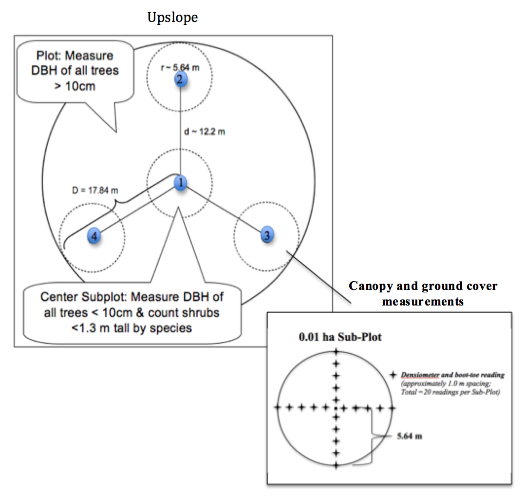
Layout of sample plots used in the Baseline Landscape Assessment. DBH = Diameter of the tree trunk at breast height (1.3 meters)
Progress
I am currently wrapping up analysis of the baseline landscape assessment (BLA) while using this information to plan the remaining activities and refine the research questions presented above. Below are highlights and figures of the preliminary BLA results for several indicators of ecosystem services, soil quality and land degradation, as well as general landscape features. More results from the BLA and other activities within this research project will be posted as they become available.
To view results, click the subcategory below each header (e.g. “Land Use and Land Cover”) and the section will expand to reveal results. Click the subcategory again to hide the results.
Baseline Landscape Assessment – Preliminary Results
Highlights:
- The most common land use/cover classes were Forest, Wooded Grassland and Agroforest
- 63% of all plots were cultivated or managed in some way
- Evidence of recent burning was observed on 27% of all sites
- 31% of Forest sites and 85% of Bush/Shurbland sites showed evidence of tree cutting
- The most commonly grown crops were sorghum, maize and beans
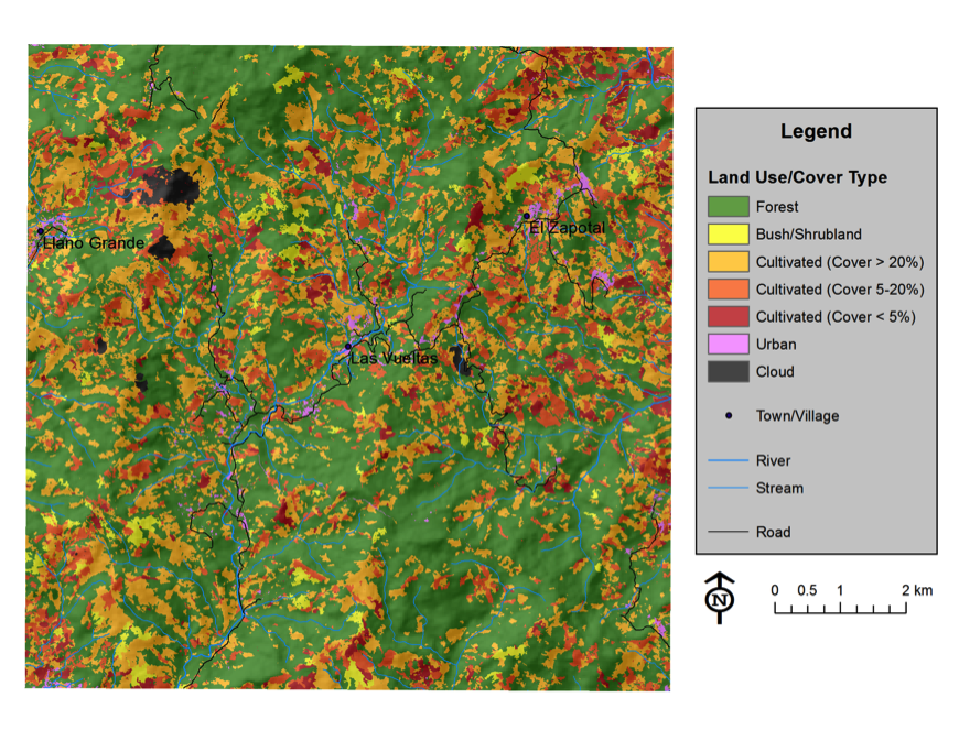
High-resolution (2.4m) map depicting the heterogeneous land use/cover across the BLA project area
A recently published dataset from Hansen et al. (2013) was used to estimate the change in tree cover from the period 2000 – 2012 (click here for a link to the global dataset). Within the BLA area, tree cover in 2000 was 4,513.84 ha or about 45% of the total area. Between 2000 and 2012 an estimated 185.72 ha of tree cover was lost with just 4.16 ha gained, totaling a net loss of 181.56 ha or 4.02% of all tree cover. Looking at the map below, we can see that the majority of forest loss is occurring at lower elevations just east of Las Vueltas and El Zapotal. Looking at the LULC map in above, this area coincides with one of the more intensively cultivated areas for cropland and pasture.
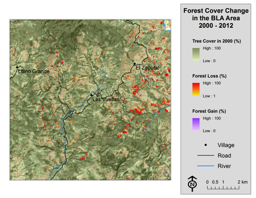
Loss of tree cover across the BLA area estimated with data published by Hansen et al. (2013) using Landsat satellite imagery
Highlights:
- Over ¾ of all sample sites had slopes classified as steep, with an average slope of 49%
- Remote sensing analysis showed that about 64% of all slopes were steep
- Slope did not vary significantly by LULC class and all classes had mean slopes of at least 39%.
- Cropland and Grassland sites were among those with the steepest slopes averaging 57% and 51%, respectively.
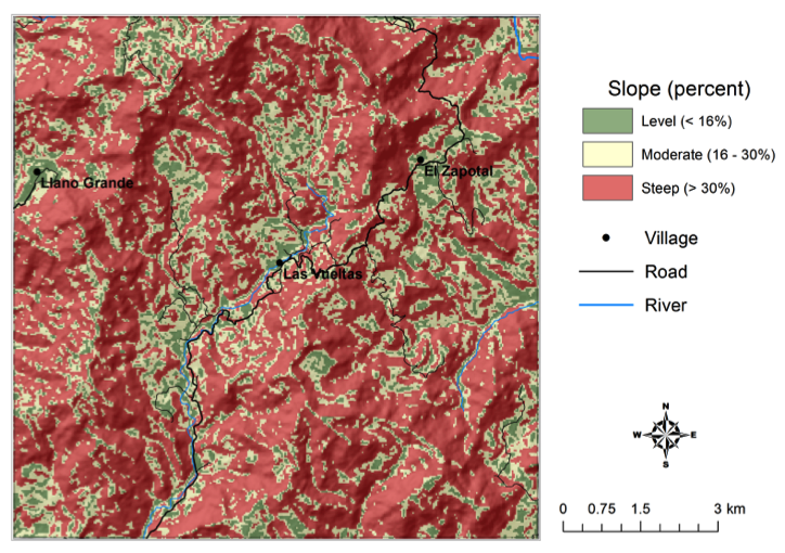
Estimated slope across the BLA area using ASTER 30m digital elevation model (DEM)
| Slope class | Sampled sites | Remote sensing |
| Level (< 16%) | 6.29% | 10.55% |
| Moderate (16 – 30%) | 16.78% | 25.08% |
| Steep (> 30%) | 76.92% | 64.37% |
| LULC Class | n | Mean Slope (%) | |
| Agroforest | 20 | 39.20 | ± 17.11 |
| Bush/Shrubland | 13 | 52.54 | ± 22.18 |
| Cropland | 12 | 56.92 | ± 23.67 |
| Forest | 64 | 48.97 | ± 24.96 |
| Grassland | 13 | 50.92 | ± 21.18 |
| Wooded Grassland | 21 | 49.24 | ± 18.02 |
A variety of soil chemical properties were analyzed to help determine soil quality, fertility and degradation. Properties analyzed include organic matter (SOM), total carbon (C), total nitrogen (N), extractable phosphorus (P), potassium (K), exchangeable calcium (exch-Ca) and magnesium (exch-Mg), zinc (Zn) and pH.
Highlights:
- Soils were surprisingly rich in soil organic matter (SOM) and carbon (C)
- Very low levels of phosphorus (P) were widespread, but the lower-lying areas in the east had adequate to very high soil P
- Potassium (K) and magnesium (Mg) may be deficient in isolated regions
- Soils were somewhat acidic (average pH of 5.61) but not to the degree found in many tropical areas and does not appear to be a widespread problem
- Elevation is highly correlated with many chemical properties
- LULC and slope do not appear to be a major determinant of soil chemical properties, with the possible exception of K
- Wooded Grassland sites tended to be the of the poorest soil quality, but likely due more to location than cause and effect
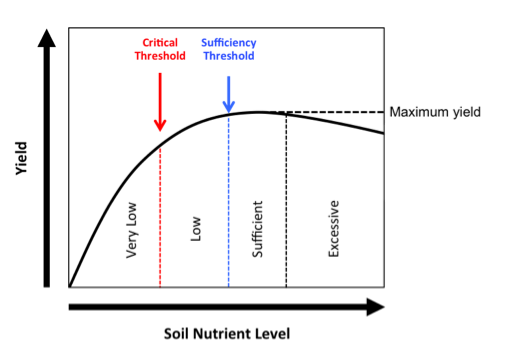
Theoretical framework for soil nutrient threshold values in relation to agricultural productivity
For each chemical soil property, we identified two key thresholds, when possible, below which agricultural productivity is likely constrained. The first is the Sufficiency Threshold. When a measured soil nutrient result lies below this level that soil is low in that nutrient and some benefit in crop productivity will likely be realized by managing for that nutrient. The second is the Critical Threshold, below which the soil is very low in that nutrient and productivity is likely to be highly constrained. Acute management of that nutrient will usually lead to large productivity gains, provided that other critically low nutrients or constraints do not exist or are adequately managed. The theoretical framework of where these thresholds lie on a yield response curve is shown to the right. Below is an example of analysis results for soil phosphorus (P) to show how soil properties can be mapped and how thresholds can be used to identify potential nutrient deficiencies.
Soil Phosphorus Results
Phosphorus is an essential plant element involved in many growth processes, especially energy storage and transfer and root development (Havlin et al., 2005). It is critical for photosynthesis and adequate P can improve the quality of harvestable products, promote nitrogen fixation in legumes, increase stalk strength and raise the tolerance of grains to root diseases. The association between adequate P and enhanced root growth can improve plant uptake of other nutrients and water, thereby reducing potential drought stress.
The amount of P available to plants is generally much lower than the total P present in the soil. P deficiency is often a problem in reddish, clayey tropical soils as these soils tend to hold most of their P in a form that is not available to plants. In this study, P was measured as an estimate of plant-available phosphorus using the Mehlich-1 extraction method. CENTA suggests that maize and bean production may be limited when available soil P is below the sufficiency threshold of 22 mg kg-1 with critical deficiencies likely below 13 mg kg-1.
Analysis of sampled soils for phosphorus yielded showed highly varied results with extractable P ranging from 1 to 446 mg kg-1. While mean P (28.9 mg kg-1)was above the sufficiency threshold, the standard deviation was more than double the mean and results were highly skewed due to a handful of samples with very high P. In general, P values were low with 80% of all samples were below the sufficiency threshold and over three-quarters below the critical threshold. In fact, more than 44% of all topsoil samples had very low P levels below 4 mg kg-1. Predicted (mapped) topsoil P across the project area ranged from 2 to 172 mg kg-1. Low P levels were predicted across the entire region with the exception of the low-lying central eastern area just north of San José Las Flores (not shown) where very high P levels were observed. Probability maps for P levels below key thresholds show that widespread P deficiencies are probable, especially west of the Las Vueltas road.
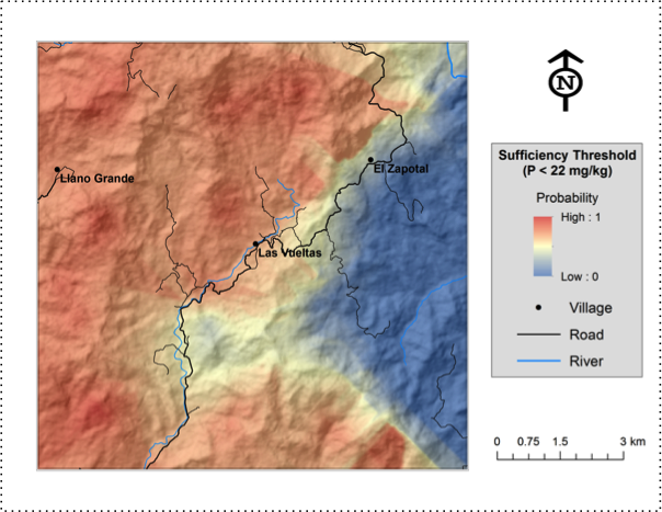
Probability map depicting the likelihood that Topsoil (0-20 cm) extractable P values are below the sufficiency threshold of 22 mg kg-1
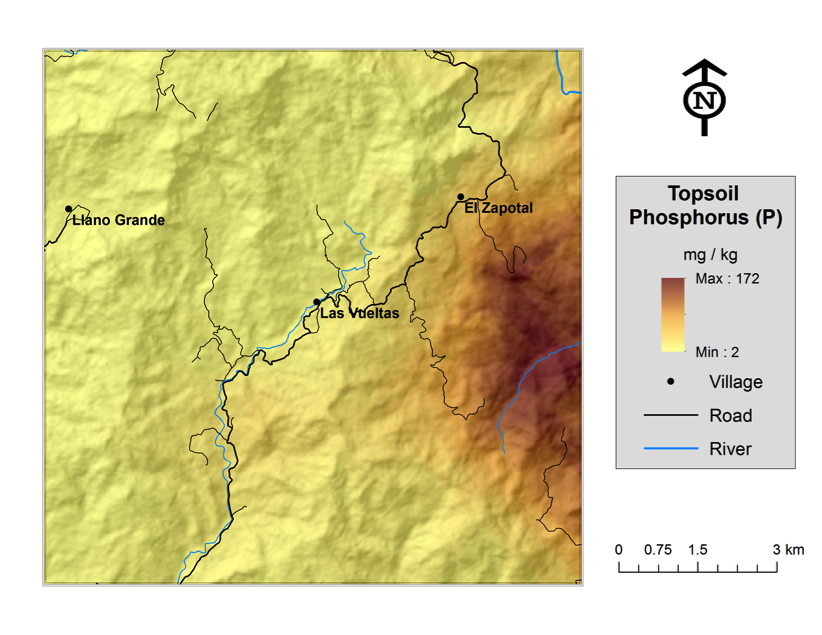
Prediction map for topsoil extractable P levels using QuickBird-derived EVI and ASTER 30m DEM layers as co-variates
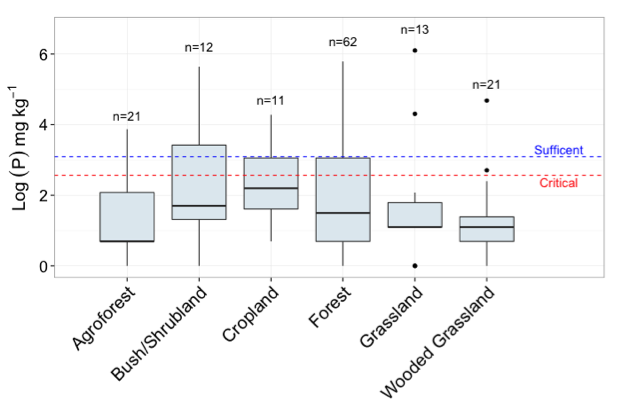
Boxplot of log-transformed topsoil P levels by LULC class
Statistical analysis was performed after a natural log transformation of phosphorus values to improve normality and presentation clarity. Mean phosphorus levels below the critical threshold were seen across all LULC classes. The lowest mean P was observed for Agroforest and Grassland sites and the highest means on Cropland, although no statistically significant differences between LULC classes were found. P did not vary significantly by percent slope or slope class (not shown). P was, however, very strongly correlated with elevation with the highest P levels found at the lowest elevations, below about 700-800m. Above this elevation, nearly all sample sites were found to have soil P below the critical threshold value of 13 mg kg-1.
There is widespread need to manage for P, especially at higher elevations. However, required additions of P are unlikely to be the same for all locations. For example, the central-eastern zone of the BLA area may require little or no P amendments, while other areas have almost no plant-available P and would require the maximum recommended application. Soil testing for P is therefore highly recommended whenever possible in order to reduce costs and avoid over-application, which could lead to polluted surface waters due to nutrient runoff. In the absence of soil testing, it can be difficult to decide how to manage for P since it is needed earlier on in plant growth. One option could be to apply a partial application of P at planting and then monitor plants for deficiencies to decide if an additional application is needed. Deficiency symptoms tend to appear as overall stunting of the plant and as a darkening of the leaves, beginning with the oldest leaves first (Havlin et al., 2005). In maize, purple leaf coloration is common when plants are deficient in P.
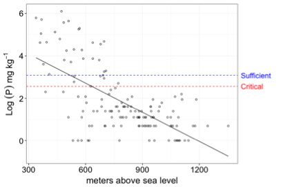
Scatterplot of log-transformed topsoil P by elevation (r = 0.66; p-value < 0.001)
P-losses may be more of a concern for this area than P adsorption. Soils in this area tend to be relatively sandy and P is therefore not held as tightly in the soil making it more susceptible to losses through surface runoff and leaching. Additionally, soils are not overly acidic and therefore less likely to adsorb added P to the point of making it unavailable to plants. These factors, combined with the high levels of SOM, indicate that plants should respond to additions of P when levels are low. Leaving crop/tree residues on the soil as a mulch and adding animal and green manures can both help increase SOM and organic P sources to increase P levels over time in sandy soils.
Physical properties analyzed were soil particle size distribution (sand, silt and clay fractions), soil depth to auger restriction and water infiltration rate.
Highlights:
- Soil depths to augur restriction varied widely with an average of about 57 cm
- The dominant soils are in the BLA area are Sandy Clay Loams (73%) and Sandy Loams (24%)
- Sand contents were high and ranged from 0.51 to 0.77
- Infiltration rates indicate that the vast majority of soils are susceptible to moderate runoff risk
Below is a map of predicted water infiltration rate across the area, an example of the kinds of maps developed related to soil physical properties.
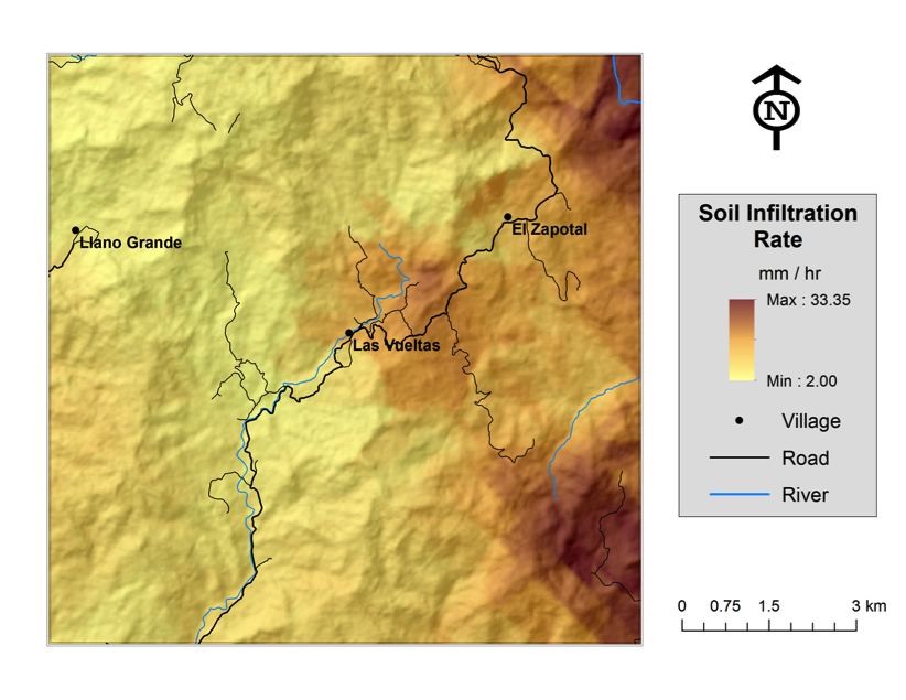
Prediction map for soil infiltration rates using QuickBird Band 1 and Insolation as co-variates
A normalized topsoil constraint index (NTCI) was calculated using select soil physical and chemical properties to evaluate the magnitude to which soils in the BLA may be constrained for agricultural productivity. The index was calculated based on the probability that soils failed to meet Sufficiency Thresholds for the seven soil properties for which data was available and thresholds could be identified (N, P, K, Ca, Mg, pH and infiltration rate) as well as soil depth and SOM. In short, the NTCI ranges from 0 (least likely to be constrained) to 100 (most likely to be constrained). If a soil at a given point had a high probability of not exceeding the Sufficiency Threshold for all seven soil properties, had a relatively shallow depth and low SOM value it would receive a score near 100. If a soil had a low probability of values below the Sufficiency Thresholds, was relatively deep and with high SOM, it would receive a score near 0. A detailed description of how the NTCI was derived is given below.
Topsoil constraint scores ranged from 16.51 to 100 with an average score of 55.72. The most highly constrained soils are predicted to be in the southwest of the BLA area between Llano Grande, Las Vueltas and Chalatenango and in the far north (see map below). The least constrained soils were predicted east of the Las Vueltas road in the lower-lying areas around El Zapotal and south toward San Jose Las Flores and in a small band between Llano Grande and El Zapotal, north of Las Vueltas.
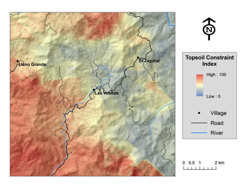
Predicted topsoil constraints to productivity based on select soil chemical and physical properties measured in the BLA
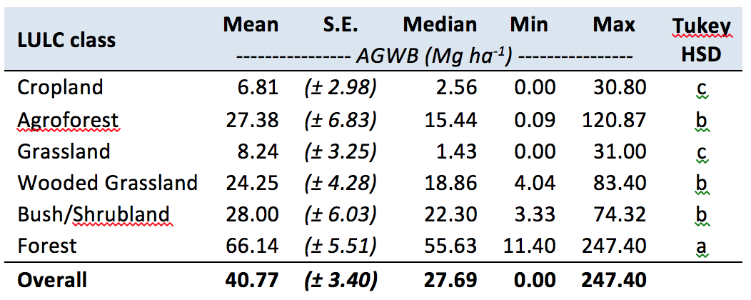
Aboveground woody biomass (AGWB) for each LULC class
Overall, aboveground woody biomass at sample sites ranged from 0 to 247.40 Mg ha-1. The highest biomass densities were found for Forest sites with average AGWB of 66.14 Mg ha-1, more than double the next highest LULC class, Bush/Shrubland (see table to the right). Agroforests, Wooded Grasslands and Bush/Shrublands all contained significantly more biomass than Cropland and Grassland sites. In fact, Agroforests held four times more biomass than Croplands and Wooded Grasslands contained about three times that of Grasslands. Biomass varied widely across Agroforest sites, ranging from near-zero to over 120 Mg ha-1, showing that Agroforests have the potential to hold nearly as much biomass as some of the Forests surveyed in this study. As described below, this is likely the result of the scarcity of large trees found in Forest sites.
AGWB was also assessed by DBH class. Despite the relatively low stem counts of large trees across the BLA study area, large trees in the top two DBH classes still contained the most biomass per hectare across most LULC types (see figure below). Overall, stem counts for trees in the largest DBH class (≥ 40cm) were 11.5 times lower than that for trees in the 10 – 20cm class, yet trees in the larger DBH class made up more than triple the biomass per hectare. The largest trees contain, on average, 6 times the biomass per tree compared to those with DBH 20 – 40cm, 33 times more than trees DBH 10 – 20cm and 269 times more than trees DBH < 10cm. LULC class did not have any significant impact on mean biomass per tree for any of the four DBH classes. Finally, no significant relationships were found between biomass and slope or elevation.

AGWB broken down by DBH class for each land use/cover type. The vast majority of biomass is stored in large trees, despite fewer of them existing on the landscape.
Finally, I am working to create spatially explicit maps of aboveground woody biomass. Below is a preliminary map created using multiple regression analysis to determine spectral variables from satellite imagery that are good predictors of biomass. There is significant room for improvement, but we are hopeful that maps with low uncertainty can be produced using high-resolution satellite imagery and/or LiDAR technology.
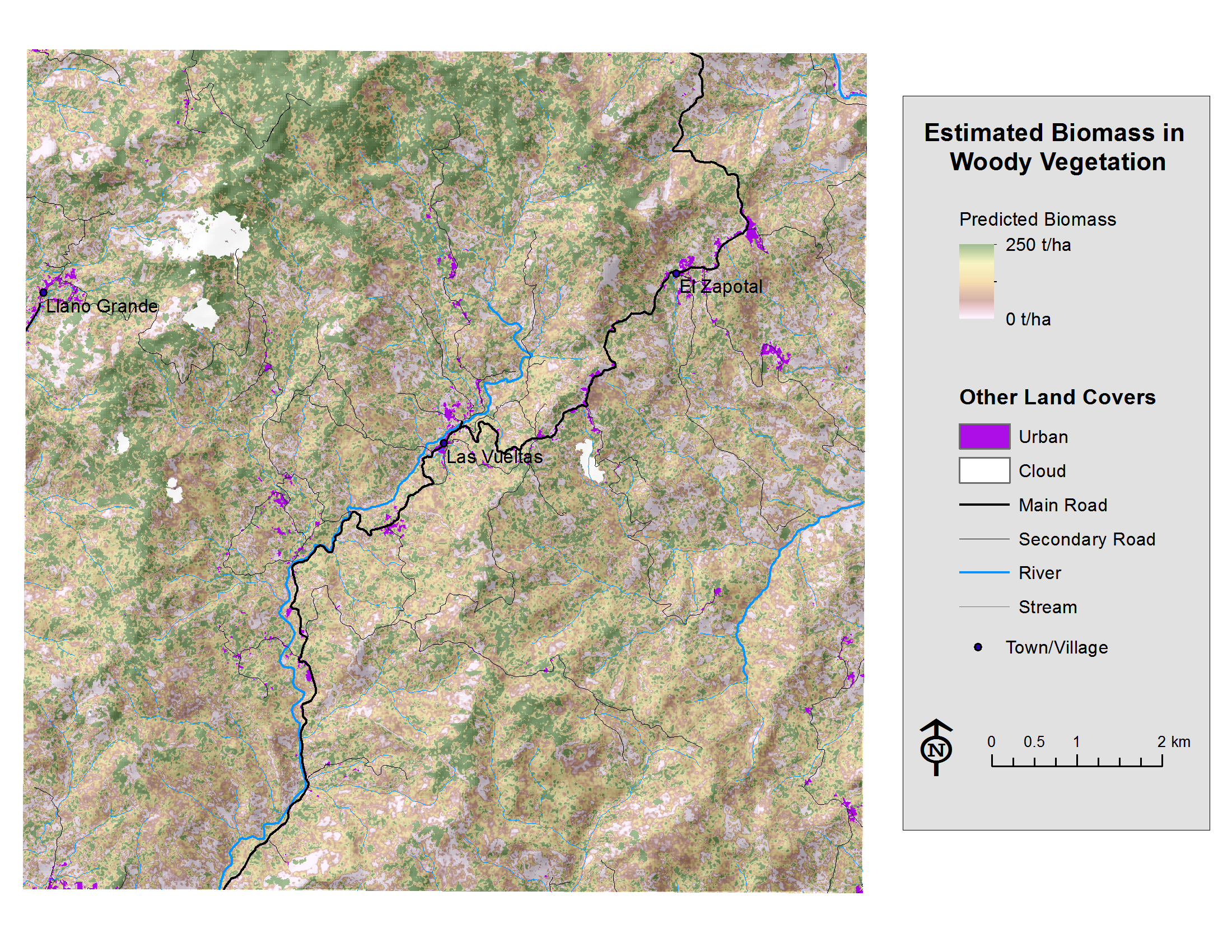
Predicted aboveground woody biomass (AGWB) across the BLA study area
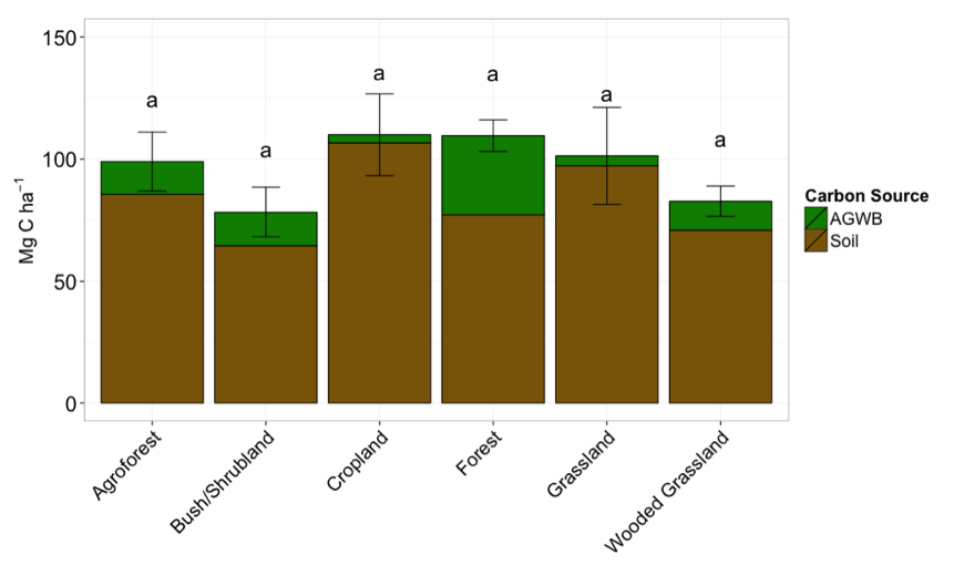
Bar chart of total carbon stocks by carbon source for all LULC classes
Total carbon stocks were calculated as the combined totals of carbon stocks stored in the soil (up to 1m depth) and in aboveground woody biomass (AGWB). Mean total carbon stocks ranged from a low of 78.42 Mg ha-1 in Bush/Shrubland sites to a high of 110.53 Mg ha-1 in Forest sites. No significant differences in total carbon were found between LULC classes when soil carbon down to 1m depth was considered. On average across the landscape, four times as much carbon was stored in the soil compared to AGWB. Soil carbon made up the largest portion of carbon stocks for Cropland sites, at 97.0%. Forest sites had the lowest proportion of soil carbon to AGWB carbon, although soils still accounted for 71.2% of total carbon stocks in Forest sites.
We also assessed the dynamic or modifiable total carbon stocks. This looks at just the carbon pools that could be reasonably altered by human management in the short to medium term (less than around 50 years), by restricting soil carbon stocks to that stored in the topsoil. Therefore, the dynamic total carbon stocks include topsoil carbon (per 1000 Mg soil) and AGWB carbon. Looking only at the dynamic carbon stocks we get a better sense of the impact of LULC class on carbon stocks and avoid some of the bias that likely exists from farmers preferentially cultivating deeper more fertile soils. Results of this analysis show that significant differences exist between LULC classes with Forests maintaining the largest carbon stocks at more than double that of the lowest classes, Cropland and Grassland. We also find that AGWB makes up a significantly larger portion of carbon stocks that could easily be affected by management. For example, in Forest sites AGWB accounts for over 73% of all dynamic carbon.
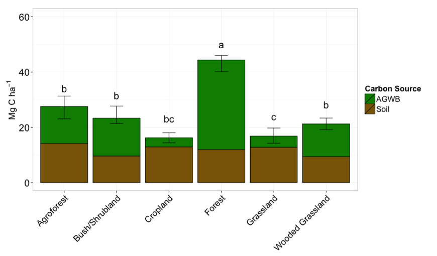
Bar chart of total dynamic carbon stocks by carbon source for all LULC classes
Spatially explicit maps of total carbon stocks are in process and will be added to this section soon!
Hansen, M.C., Potapov, P. V., Moore, R., Hancher, M., Turubanova, S. a., Tyukavina, a., Thau, D., Stehman, S. V., Goetz, S.J., Loveland, T.R., Kommareddy, a., Egorov, a., Chini, L., Justice, C.O., Townshend, J.R.G., 2013. High-Resolution Global Maps of 21st-Century Forest Cover Change. Science (80-. ). 342, 850–853.
Havlin, J.L., Beaton, J.D., Tisdale, S.L., Nelson, W.L., 2005. Soil Fertility and Fertilizers, 7th ed. Pearson Prentice Hall, Upper Saddle River, N.J.
Vågen T-G, Shepherd K D, Walsh M G, Winowiecki L A, Tamene Desta L and Tondoh J E 2010 AfSIS Technical Specifications—Soil Health Surveillance (Nairobi: CIAT (the AfSIS Project))
Visit the Photo Page to view photos of field work, the project site, participating farmers and more.